@
前言
上一篇和大家一起分享了如何使用LabVIEW OpenCV dnn实现手写数字识别,今天我们一起来看一下如何使用LabVIEW OpenCV dnn实现图像分类。
一、什么是图像分类?
1、图像分类的概念
图像分类,核心是从给定的分类集合中给图像分配一个标签的任务。实际上,这意味着我们的任务是分析一个输入图像并返回一个将图像分类的标签。标签总是来自预定义的可能类别集。
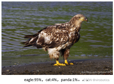
示例:我们假定一个可能的类别集categories = {dog, cat, eagle},之后我们提供一张图片(下图)给分类系统。这里的目标是根据输入图像,从类别集中分配一个类别,这里为eagle,我们的分类系统也可以根据概率给图像分配多个标签,如eagle:95%,cat:4%,panda:1%
2、MobileNet简介
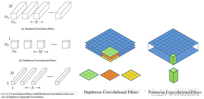
MobileNet:基本单元是深度级可分离卷积(depthwise separable convolution),其实这种结构之前已经被使用在Inception模型中。深度级可分离卷积其实是一种可分解卷积操作(factorized convolutions),其可以分解为两个更小的操作:depthwise convolution和pointwise convolution,如图1所示。Depthwise convolution和标准卷积不同,对于标准卷积其卷积核是用在所有的输入通道上(input channels),而depthwise convolution针对每个输入通道采用不同的卷积核,就是说一个卷积核对应一个输入通道,所以说depthwise convolution是depth级别的操作。而pointwise convolution其实就是普通的卷积,只不过其采用1x1的卷积核。图2中更清晰地展示了两种操作。对于depthwise separable convolution,其首先是采用depthwise convolution对不同输入通道分别进行卷积,然后采用pointwise convolution将上面的输出再进行结合,这样其实整体效果和一个标准卷积是差不多的,但是会大大减少计算量和模型参数量。
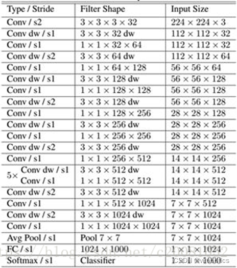
MobileNet的网络结构如表所示。首先是一个3x3的标准卷积,然后后面就是堆积depthwise separable convolution,并且可以看到其中的部分depthwise convolution会通过strides=2进行down sampling。然后采用average pooling将feature变成1x1,根据预测类别大小加上全连接层,最后是一个softmax层。如果单独计算depthwise convolution和pointwise convolution,整个网络有28层(这里Avg Pool和Softmax不计算在内)。
二、使用python实现图像分类(py_to_py_ssd_mobilenet.py)
1、获取预训练模型
- 使用tensorflow.keras.applications获取模型(以mobilenet为例);
from tensorflow.keras.applications import MobileNet
    original_tf_model = MobileNet(
        include_top=True,
        weights="imagenet"
    )
- 把original_tf_model打包成pb
def get_tf_model_proto(tf_model):
    # define the directory for .pb model
    pb_model_path = "models"

    # define the name of .pb model
    pb_model_name = "mobilenet.pb"

    # create directory for further converted model
    os.makedirs(pb_model_path, exist_ok=True)

    # get model TF graph
    tf_model_graph = tf.function(lambda x: tf_model(x))

    # get concrete function
    tf_model_graph = tf_model_graph.get_concrete_function(
        tf.TensorSpec(tf_model.inputs[0].shape, tf_model.inputs[0].dtype))

    # obtain frozen concrete function
    frozen_tf_func = convert_variables_to_constants_v2(tf_model_graph)
    # get frozen graph
    frozen_tf_func.graph.as_graph_def()

    # save full tf model
    tf.io.write_graph(graph_or_graph_def=frozen_tf_func.graph,
                      logdir=pb_model_path,
                      name=pb_model_name,
                      as_text=False)

    return os.path.join(pb_model_path, pb_model_name)
2、使用opencv_dnn进行推理
- 图像预处理(blob)
def get_preprocessed_img(img_path):
    # read the image
    input_img = cv2.imread(img_path, cv2.IMREAD_COLOR)
    input_img = input_img.astype(np.float32)

    # define preprocess parameters
    mean = np.array([1.0, 1.0, 1.0]) * 127.5
    scale = 1 / 127.5

    # prepare input blob to fit the model input:
    # 1. subtract mean
    # 2. scale to set pixel values from 0 to 1
    input_blob = cv2.dnn.blobFromImage(
        image=input_img,
        scalefactor=scale,
        size=(224, 224),  # img target size
        mean=mean,
        swapRB=True,  # BGR -> RGB
        crop=True  # center crop
    )
    print("Input blob shape: {}\n&