lpha <- runif(1)
beta <- runif(1)
while (alpha + beta >= up_limit)
{
alpha <- runif(1)
beta <- runif(1)
}
return(
list(omega = omega, alpha = alpha, beta = beta))
}
train_length <- 3000
val_length <- 1000
test_length <- 1000
train_m1 <- numeric(train_length)
train_m2 <- numeric(train_length)
train_m1_5 <- numeric(train_length)
train_omega <- numeric(train_length)
train_alpha <- numeric(train_length)
train_beta <- numeric(train_length)
val_m1 <- numeric(val_length)
val_m2 <- numeric(val_length)
val_m1_5 <- numeric(val_length)
val_omega <- numeric(val_length)
val_alpha <- numeric(val_length)
val_beta <- numeric(val_length)
test_m1 <- numeric(test_length)
test_m2 <- numeric(test_length)
test_m1_5 <- numeric(test_length)
生成训练数据。
# Train Data ----

for (i in 1:train_length)
{
    garch_coef <- GarchCoefGenerator()
    garch_sample <- garchSim(
        garchSpec(
            model = garch_coef),
        n.start = 1000, n = 1000)

    train_m1[i] <- M1(garch_sample)
    train_m2[i] <- M2(garch_sample)
    train_m1_5[i] <- M1_5(garch_sample)

    train_omega[i] <- garch_coef$omega
    train_alpha[i] <- garch_coef$alpha
    train_beta[i] <- garch_coef$beta
}

trainX <- data.frame(
    m1 = train_m1,
    m2 = train_m2,
    m1_5 = train_m1_5) %>%
    as.matrix()

trainY <- data.frame(
    omega = train_omega,
    alpha = train_alpha,
    beta = train_beta) %>%
    as.matrix()
生成验证数据。
# Val Data ----

for (i in 1:val_length)
{
    garch_coef <- GarchCoefGenerator()
    garch_sample <- garchSim(
        garchSpec(
            model = garch_coef),
        n.start = 1000, n = 1000)

    val_m1[i] <- M1(garch_sample)
    val_m2[i] <- M2(garch_sample)
    val_m1_5[i] <- M1_5(garch_sample)

    val_omega[i] <- garch_coef$omega
    val_alpha[i] <- garch_coef$alpha
    val_beta[i] <- garch_coef$beta
}

valX <- data.frame(
    m1 = val_m1,
    m2 = val_m2,
    m1_5 = val_m1_5) %>%
    as.matrix()

valY <- data.frame(
    omega = val_omega,
    alpha = val_alpha,
    beta = val_beta) %>%
    as.matrix()
用 keras 构建神经网络。
# Model Training ----

model <- keras_model_sequential()

model %>%
    layer_dense(
        units = 9,
        input_shape = c(3),
        activation = 'sigmoid') %>%
    layer_dense(
        units = 3,
        activation = 'sigmoid') %>%
    compile(
        loss = 'mae',
        optimizer = 'adam')

summary(model)
实验采用了结构非常简单的神经网络结构,一个两层的多元感知机,超参数、激活函数和优化方法没有调优。
__________________________________________________________________________
Layer (type)                     Output Shape                 Param #
==========================================================================
dense_1 (Dense)                  (None, 9)                    36
__________________________________________________________________________
dense_2 (Dense)                  (None, 3)                    30
==========================================================================
Total params: 66
Trainable params: 66
Non-trainable params: 0
__________________________________________________________________________
训练。
history <- model %>%
fit(
trainX,
trainY,
validation_data = list(
valX, valY),
batch_size = 50,
epochs = 1000)
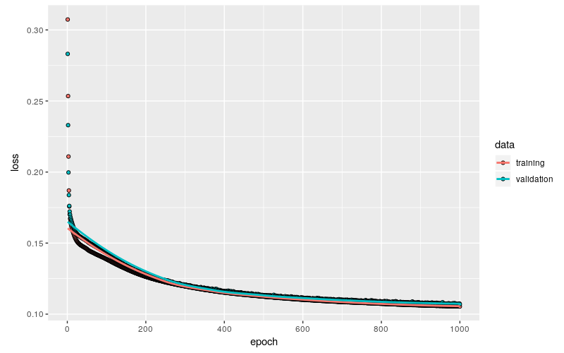
plot(history)
训练结果非常理想,训练集和验证集上的 loss 基本上同步衰减到 0.11 左右,并且从趋势上看大约已经接近了极限水平。
延续前面两篇博文的主题,将 \(\text{GARCH}(1,1)\) 的模型参数限定为 \((0.2,0.2,0.2)\),生成测试数据,后面要测试估计值的稳定性,以及是否有偏。
# Test ----

for (i in 1:test_length)
{
    garch_coef <- list(
        omega = 0.2, alpha = 0.2, beta = 0.2)