lo.95 hi.80 hi.95
## <date> <chr> <dbl> <dbl> <dbl> <dbl> <dbl>
## 1 2010-01-01 actual 6558 NA NA NA NA
## 2 2010-02-01 actual 7481 NA NA NA NA
## 3 2010-03-01 actual 9475 NA NA NA NA
## 4 2010-04-01 actual 9424 NA NA NA NA
## 5 2010-05-01 actual 9351 NA NA NA NA
## 6 2010-06-01 actual 10552 NA NA NA NA
## 7 2010-07-01 actual 9077 NA NA NA NA
## 8 2010-08-01 actual 9273 NA NA NA NA
## 9 2010-09-01 actual 9420 NA NA NA NA
## 10 2010-10-01 actual 9413 NA NA NA NA
## # ... with 86 more rows
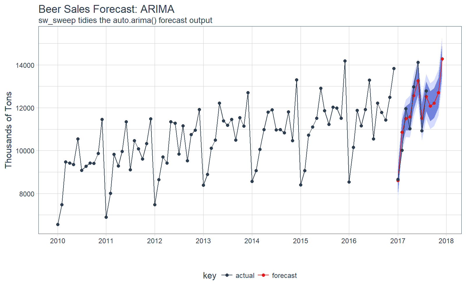
STEP 5:比较真实值和预测值
我们可以使用 tq_get() 来检索实际数据。注意,我们没有用于比较的完整数据,但我们至少可以比较前几个月的实际值。
actuals_tbl <- tq_get(
    "S4248SM144NCEN",
    get = "economic.data",
    from = "2017-01-01",
    to = "2017-12-31")
注意,预测结果放在 tibble 中,可以方便的实现可视化。
# Visualize the forecast with ggplot
fcast_tbl %>%
    ggplot(
        aes(x = index, y = price, color = key)) +
    # 95% CI
    geom_ribbon(
        aes(ymin = lo.95, ymax = hi.95),
        fill = "#D5DBFF", color = NA, size = 0) +
    # 80% CI
    geom_ribbon(
        aes(ymin = lo.80, ymax = hi.80, fill = key),
        fill = "#596DD5", color = NA,
        size = 0, alpha = 0.8) +
    # Prediction
    geom_line() +
    geom_point() +
    # Actuals
    geom_line(
        aes(x = date, y = price), color = palette_light()[[1]],
        data = actuals_tbl) +
    geom_point(
        aes(x = date, y = price), color = palette_light()[[1]],
        data = actuals_tbl) +
    # Aesthetics
    labs(
        title = "Beer Sales Forecast: ARIMA", x = "", y = "Thousands of Tons",
        subtitle = "sw_sweep tidies the auto.arima() forecast output") +
    scale_x_date(
        date_breaks = "1 year",
        date_labels = "%Y") +
    scale_color_tq() +
    scale_fill_tq() +
    theme_tq()
我们可以研究测试集上的误差(真实值 vs 预测值)。
# Investigate test error
error_tbl <- left_join(
    actuals_tbl,
    fcast_tbl,
    by = c("date" = "index")) %>%
    rename(
        actual = price.x, pred = price.y) %>%
    select(date, actual, pred) %>%
    mutate(
        error     = actual - pred,
        error_pct = error / actual)

error_tbl
## # A tibble: 8 x 5
##         date actual      pred      error    error_pct
##       <date>  <int>     <dbl>      <dbl>        <dbl>
## 1 2017-01-01   8664  8601.815   62.18469  0.007177365
## 2 2017-02-01  10017 10855.429 -838.42908 -0.083700617
## 3 2017-03-01  11960 11502.214  457.78622  0.038276439
## 4 2017-04-01  11019 11582.600 -563.59962 -0.051147982
## 5 2017-05-01  12971 12566.765  404.23491  0.031164514
## 6 2017-06-01  14113 13263.918  849.08191  0.060163106
## 7 2017-07-01  10928 11507.277 -579.27693 -0.053008504
## 8 2017-08-01  12788 12527.278  260.72219  0.020388035
并且,我们可以做简单的误差度量。MAPE 接近 4.3%,比简单的线性回归模型略好一点,但是 RMSE 变差了。
# Calculate test error metrics
test_residuals <- error_tbl$error
test_error_pct <- error_tbl$error_pct * 100 # Percentage error

me   <- mean(test_residuals, na.rm=TRUE)
rmse <- mean(test_residuals^2, na.rm=TRUE)^0.5
mae  <- mean(abs(test_residuals), na.rm=TRUE)
mape <- mean(abs(test_error_pct), na.rm=TRUE)
mpe  <- mean(test_error_pct, na.rm=TRUE)

tibble(me, rmse, mae, mape, mpe) %>%
    glimpse()
## Observations: 1
## Variables: 5
## $ me   <dbl> 6.588034
## $ rmse <dbl> 561.4631
## $ mae  <dbl> 501.9144
## $ mape <dbl> 4.312832
## $ mpe  <dbl> -0.3835956