和金融数据一样，使用 ggplot2 画图，使用 tidyquant 提供的主题（调用 theme_tq() 和 scale_color_tq()）实现金融、商务风格的可视化效果。

# Plot data
FRED_data_m %>%
    ggplot(aes(x = date, y = price, color = symbol)) + 
    geom_line() +
    facet_wrap(~ symbol, ncol = 2, scales = "free_y") +
    theme_tq() +
    scale_color_tq() +
    labs(title = "Visualize Economic Data")

使用 tq_transmute 和 tq_mutate 转换数据

函数 tq_transmute() 和 tq_mutate() 可以使 xts、zoo 和 quantmod 中的函数调用更“tidy”。这里直接介绍使用，“可用函数”一节罗列了已经整合进 tidyquant 的若干其他函数。

tq_transmute

tq_transmute() 与 tq_mutate() 之间的区别在于 tq_transmute() 将返回一个新的数据框对象，而 tq_mutate() 则在原有数据框的基础上横向添加数据（例如，增加一列）。当数据因为改变周期而改变行数时，tq_transmute() 特别有用。

改变周期与 tq_transmute

下面的例子将改变数据的周期，从每日数据变为月度数据。这时，你需要使用 tq_transmute() 来完成这一操作，因为数据的行数改变了。

# Change periodicity from daily to monthly using to.period from xts
FANG_data_m <- FANG_data_d %>%
    group_by(symbol) %>%
    tq_transmute(
        select      = adjusted,
        mutate_fun  = to.period,
        period      = "months")

FANG_data_m

## # A tibble: 144 x 3
## # Groups:   symbol [4]
##    symbol       date adjusted
##     <chr>     <date>    <dbl>
##  1     FB 2014-01-31    62.57
##  2     FB 2014-02-28    68.46
##  3     FB 2014-03-31    60.24
##  4     FB 2014-04-30    59.78
##  5     FB 2014-05-30    63.30
##  6     FB 2014-06-30    67.29
##  7     FB 2014-07-31    72.65
##  8     FB 2014-08-29    74.82
##  9     FB 2014-09-30    79.04
## 10     FB 2014-10-31    74.99
## # ... with 134 more rows

改变数据周期可以缩减数据量。一些注意事项项：

• theme_tq() 和 scale_color_tq() 用来绘制商务风格的图。
• 如果要改变数据的周期或者进行其他基于时间的操作，请留意后续关于 tibbletime 包的教程，tibbletime 以另外一种标准处理基于时间的操作。

周期改变前，数据太多

# Daily data
FANG_data_d %>%
    ggplot(aes(date, adjusted, color = symbol)) +
    geom_point() +
    geom_line() +
    facet_wrap(~ symbol, ncol = 2, scales = "free_y") +
    scale_color_tq() +
    theme_tq() +
    labs(title = "Before transformation: Too Much Data")

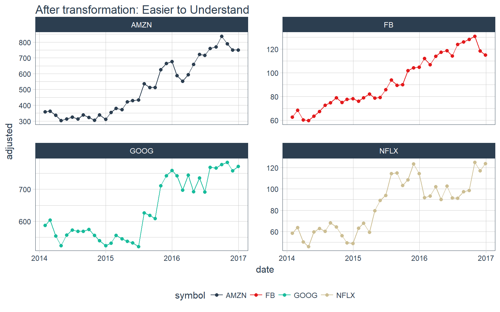
周期改变后，容易理解

用 tq_transmute() 转变成月度数据后容易理解多了。

# Monthly data
FANG_data_m %>%
    ggplot(aes(date, adjusted, color = symbol)) +
    geom_point() +
    geom_line() +
    facet_wrap(~ symbol, ncol = 2, scales = "free_y") +
    scale_color_tq() +
    theme_tq() +
    labs(title = "After transformation: Easier to Understand")

tq_mutate

tq_mutate() 函数基于 xts 包为数据添加新的列。正因为这样，当返回数据不止一列时，tq_mutate() 显得特别有用（dplyr::mutate() 就没有这样的功能）。

tq_mutate 与滞后数据

一个关于 lag.xts 的例子。通常我们需要不只一列滞后数据，这正是 tq_mutate() 擅长的。下面，为原数据添加五列滞后数据。

# Lags - Get first 5 lags

# Pro Tip: Make the new column names first, then add to the `col_rename` arg
column_names <- paste0("lag", 1:5)

# First five lags are output for each group of symbols
FANG_data_d %>%
    select(symbol, date, adjusted) %>%
    group_by(symbol) %>%
    tq_mutate(
        select     = adjusted,
        mutate_fun = lag.xts,
        k          = 1:5,
        col_rename = column_names)