rdized Root Mean Square Residual:
SRMR 0.065
#以下是参数估计部分
Parameter Estimates:
Information Expected
Standard Errors Standard
Latent Variables:
Estimate Std.Err z-value P(>|z|)
visual =~
x1 1.000
x2 0.554 0.100 5.554 0.000
x3 0.729 0.109 6.685 0.000
textual =~
x4 1.000
x5 1.113 0.065 17.014 0.000
x6 0.926 0.055 16.703 0.000
speed =~
x7 1.000
x8 1.180 0.165 7.152 0.000
x9 1.082 0.151 7.155 0.000
Covariances:
Estimate Std.Err z-value P(>|z|)
visual ~~
textual 0.408 0.074 5.552 0.000
speed 0.262 0.056 4.660 0.000
textual ~~
speed 0.173 0.049 3.518 0.000
Variances:
Estimate Std.Err z-value P(>|z|)
.x1 0.549 0.114 4.833 0.000
.x2 1.134 0.102 11.146 0.000
.x3 0.844 0.091 9.317 0.000
.x4 0.371 0.048 7.779 0.000
.x5 0.446 0.058 7.642 0.000
.x6 0.356 0.043 8.277 0.000
.x7 0.799 0.081 9.823 0.000
.x8 0.488 0.074 6.573 0.000
.x9 0.566 0.071 8.003 0.000
visual 0.809 0.145 5.564 0.000
textual 0.979 0.112 8.737 0.000
speed 0.384 0.086 4.451 0.000
例1是一个定义模型、拟合模型、提取结果的过程。
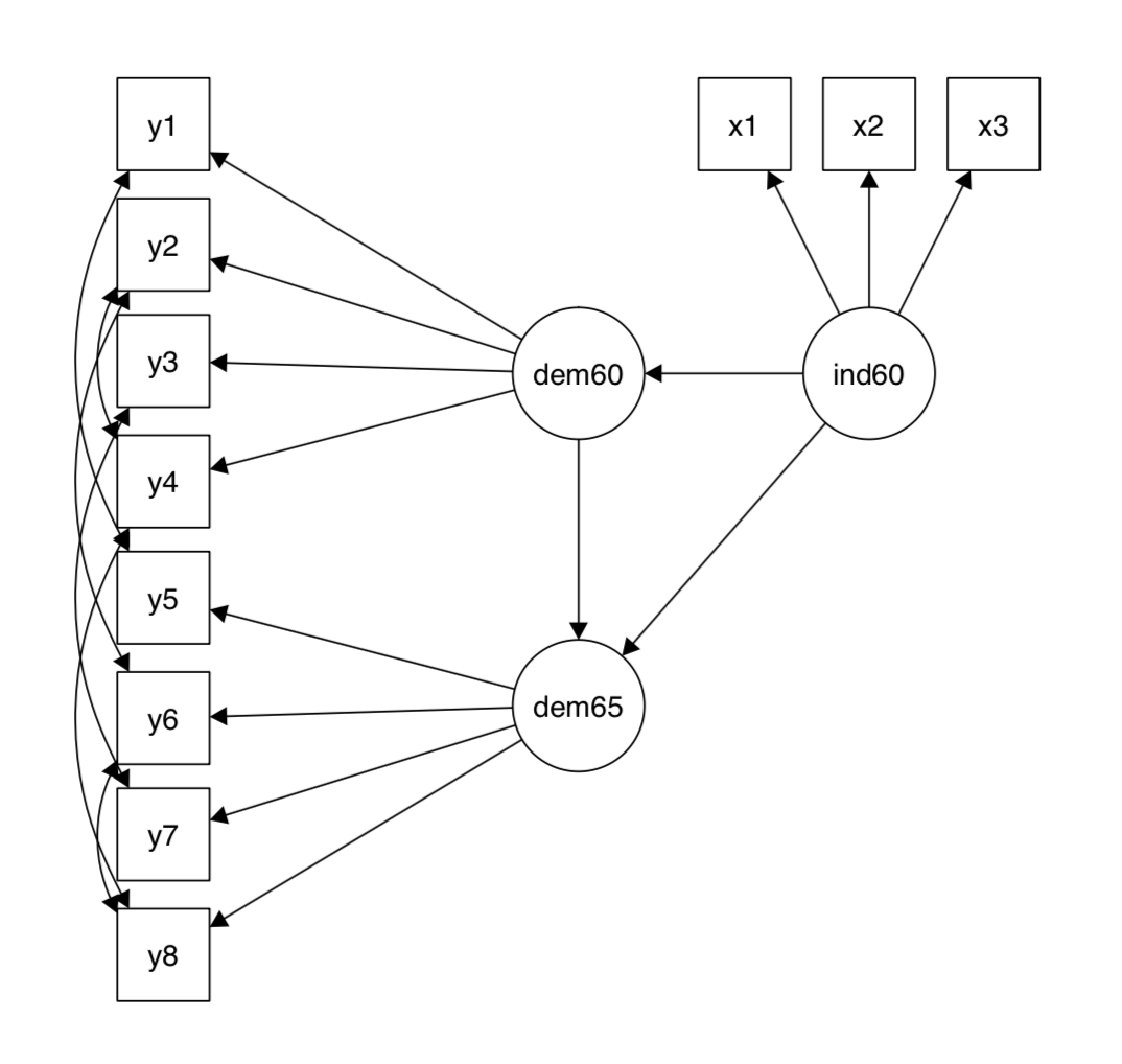
5. 例2:结构方程(SEM)
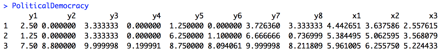
例2中我们使用名为PoliticalDemocracy的数据集,图示如下:
数据形式大致如下(只显示前三行):
| ind60 |
1960年的非民主情况 |
y5 |
1965年专家对出版物自由的评价 |
| dem60 |
1960年的民主情况 |
y6 |
1965年的反对党派自由 |
| dem65 |
1965年的民主情况 |
y7 |
1965年选举的公平性 |
| y1 |
1960年专家对出版物自由的评价 |
y8 |
1965年选举产生的立法机关效率 |
| y2 |
1960年的反对党派自由 |
x1 |
1960年每单位资本GNP |
| y3 |
1960年选举的公平性 |
x2 |
1960年每单位资本的物质能量消费 |
| y4 |
1960年选举产生的立法机关效率 |
x3 |
1960年工业劳动力占比 |
模型如下:
model <- '# measurement model 测量模型
          ind60 =~ x1 + x2 + x3
          dem60 =~ y1 + y2 + y3 + y4
          dem65 =~ y5 + y6 + y7 + y8

          # regressions 回归
          dem60 ~ ind60
          dem65 ~ ind60 + dem60

          # residual correlations 残余相关
          y1 ~~ y5
          y2 ~~ y4 + y6
          y3 ~~ y7
          y4 ~~ y8
          y6 ~~ y8'

# 拟合SEM
fit <- sem(model, data = PoliticalDemocracy)

# 提取结果
summary(fit, standardized = TRUE)

#与上例不同,这里我们忽略了参数fit.measure = TRUE,用standardized = TRUE来标准化参数值)
结果如下:
lavaan (0.5-23.1097) converged normally after  68 iterations

  Number of observations                            75

  Estimator                                         ML
  Minimum Function Test Statistic               38.125
  Degrees of freedom                                35
  P-value (Chi-square)                           0.329

Parameter Estimates:

  Information                                 Expected
  Standard Errors                             Standard

Latent Variables:
                   Estimate  Std.Err  z-value  P(>|z|)   Std.lv  Std.all
  ind60 =~
    x1                1.000                               0.670    0.920
    x2                2.180    0.139   15.742    0.000    1.460    0.973
    x3                1.819    0.152   11.967    0.000    1.218    0.872
  dem60 =~
    y1                1.000                               2.223    0.850
    y2                1.257    0.182    6.889    0.000    2.794    0.717
    y3                1.058    0.151    6.987    0.000    2.351    0.722
    y4                1.265    0.145    8.722    0.000    2.812    0.846
  dem65 =~
    y5                1.000                               2.103    0.808
    y6                1.186    0.169    7.024    0.000    2.493    0.746
    y7                1.280    0.160    8.002    0.000    2.691    0.824
    y8                1.266    0.158    8.007    0.000    2.662    0.828

Regressions:
                   Estimate  Std.Err  z-value  P(>|z|)   Std.lv  Std.all
  dem60 ~
    ind60             1.483    0.399    3.715    0.000    0.447    0.447
  dem65 ~
    ind60             0.572    0.221    2.586    0.010    0.182    0.182
    dem60             0.837    0.098    8.514    0.000    0.885    0.885

Covariances:
                   Estimate  Std.Err  z-value  P(>|z|)   Std.lv  Std.all
 .y1 ~~
   .y5                0.624    0.358    1.741    0.082    0.624    0.296
 .y2 ~~
   .y4                1.313    0.702    1.871    0.061    1.313    0.273
   .y6                2.153    0.734    2.934    0.003    2.153    0.356
 .y3 ~~
   .y7                0.795    0.608    1.308    0.191    0.795    0.191
 .y4 ~~
   .y8                0.348    0.442    0.787    0.431    0.348    0.109
 .y6 ~~
   .y8                1.356    0.568    2.386    0.017    1.356    0.338

Variances:
                   Estimate  Std.Err  z-value  P(>|z|)   Std.lv  Std.all
   .x1                0.082    0.019    4.184    0.000    0.082    0.154
   .x2                0.120    0.070    1.718    0.086    0.120    0.053
   .x3                0.467    0.090    5.177    0.000    0.467    0.239
   .y1                1.891    0.444    4.256    0.000    1.891    0.277
   .y2                7.373    1.374    5.366    0.000    7.373    0.486
   .y3                5.067    0.952    5.324    0.000    5.067    0.478
   .y4                3.148    0.739    4.261    0.000    3.148    0.28