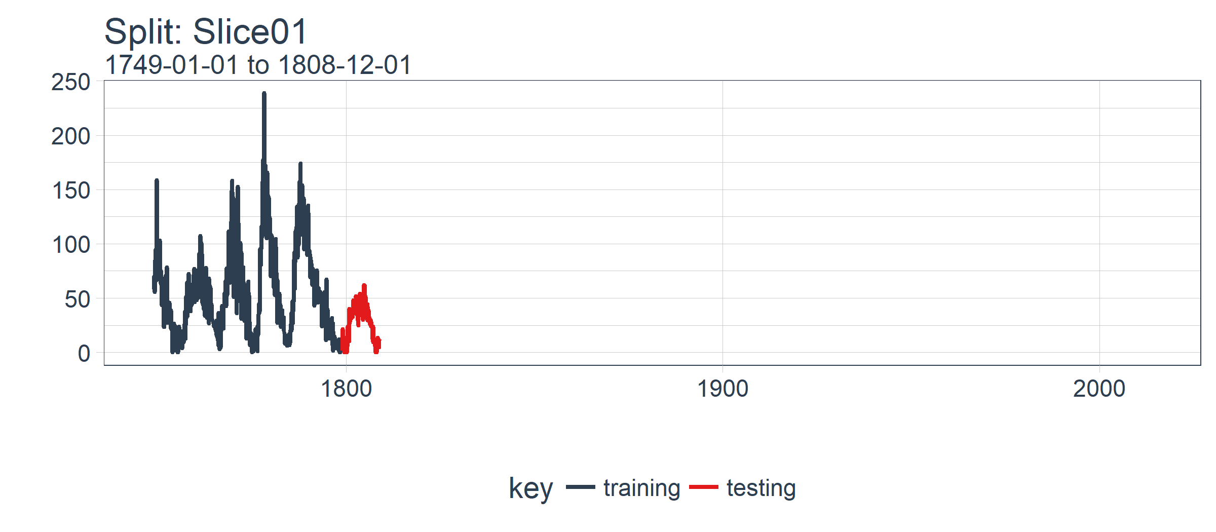
(在本例中为 Slice01),并可视化抽样策略。我们使用 expand_y_axis = TRUE 将横坐标范围扩展到整个数据集的日期范围。
rolling_origin_resamples$splits[[1]] %>%
    plot_split(expand_y_axis = TRUE) +
    theme(legend.position = "bottom")
第二个函数是 plot_sampling_plan(),使用 purrr 和 cowplot 将 plot_split() 函数应用到所有样本上。
# Plotting function that scales to all splits
plot_sampling_plan <- function(sampling_tbl,
                               expand_y_axis = TRUE,
                               ncol = 3,
                               alpha = 1,
                               size = 1,
                               base_size = 14,
                               title = "Sampling Plan") {

    # Map plot_split() to sampling_tbl
    sampling_tbl_with_plots <- sampling_tbl %>%
        mutate(
            gg_plots = map(
                splits, plot_split,
                expand_y_axis = expand_y_axis,
                alpha = alpha,
                base_size = base_size))

    # Make plots with cowplot
    plot_list <- sampling_tbl_with_plots$gg_plots

    p_temp <- plot_list[[1]] + theme(legend.position = "bottom")
    legend <- get_legend(p_temp)

    p_body  <- plot_grid(
        plotlist = plot_list, ncol = ncol)

    p_title <- ggdraw() +
        draw_label(
            title,
            size = 18,
            fontface = "bold",
            colour = palette_light()[[1]])

    g <- plot_grid(
        p_title,
        p_body,
        legend,
        ncol = 1,
        rel_heights = c(0.05, 1, 0.05))

    return(g)
}
现在我们可以使用 plot_sampling_plan() 可视化整个回测策略!我们可以看到抽样计划如何平移抽样窗口逐渐切分出训练和测试子样本。
rolling_origin_resamples %>%
    plot_sampling_plan(
        expand_y_axis = T,
        ncol = 3, alpha = 1,
        size = 1, base_size = 10,
        title = "Backtesting Strategy: Rolling Origin Sampling Plan")

此外,我们可以让 expand_y_axis = FALSE,对每个样本进行缩放。
rolling_origin_resamples %>%
    plot_sampling_plan(
        expand_y_axis = F,
        ncol = 3, alpha = 1,
        size = 1, base_size = 10,
        title = "Backtesting Strategy: Zoomed In")
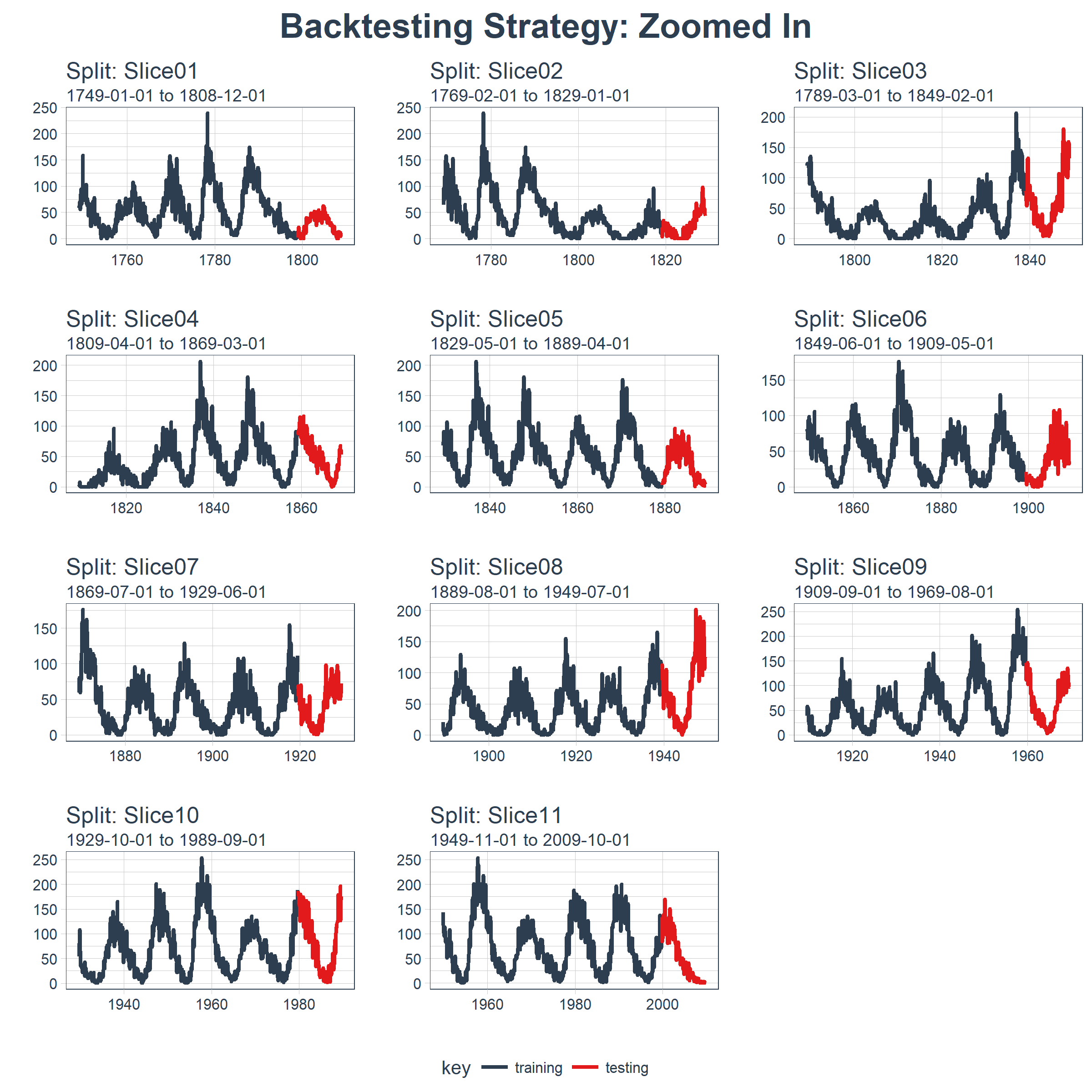
当在太阳黑子数据集上测试 LSTM 模型准确性时,我们将使用这种回测策略(来自一个时间序列的 11 个样本,每个时间序列分为 50/10 两部分,并且样本之间有 20 年的偏移)。
5 用 Keras 构建状态 LSTM 模型
首先,我们将在回测策略的某个样本上用 Keras 开发一个状态 LSTM 模型。然后,我们将模型套用到所有样本,以测试和验证模型性能。
5.1 单个 LSTM 模型
对单个 LSTM 模型,我们选择并可视化最近一期的分割样本(Slice11),这一样本包含了最新的数据。
split    <- rolling_origin_resamples$splits[[11]]
split_id <- rolling_origin_resamples$id[[11]]
5.1.1 可视化该分割样本
我么可以用 plot_split() 函数可视化该分割,设定 expand_y_axis = FALSE 以便将横坐标缩放到样本本身的范围。
plot_split(
    split,
    expand_y_axis = FALSE,
    size = 0.5) +
    theme(legend.position = "bottom") +
    ggtitle(glue("Split: {split_id}"))

5.1.2 数据准备
首先,我们将训练和测试数据集合成一个数据集,并使用列 key 来标记它们来自哪个集合(training 或 testing)。请注意,tbl_time 对象需要在调用 bind_rows() 时重新指定索引,但是这个问题应该很快在 dplyr 包中得到纠正。
df_trn <- training(split)
df_tst <- testing(split)

df <- bind_rows(
    df_trn %>% add_column(key = "training"),
    df_tst %>% add_column(key = "testing")) %>%
    as_tbl_time(index = index)

df
## # A time tibble: 720 x 3
## # Index: index
##    index      value key
##    <date>     <dbl> <chr>
##  1 1949-11-01 144.  training
##  2 1949-12-01 118.  training
##  3 1950-01-01 102.  training
##  4 1950-02-01  94.8 training
##  5 1950-03-01 110.  training
##  6 1950-04-01 113.  training
##  7 1950-05-01 106.  training
##  8 1950-06-01  83.6 training
##  9 1950-07-01  91.0 training
## 10 1950-08-01  85.2 training
## # ... with 710 more rows
5.1.3 用 recipe 做数据预处理
LSTM 算法要求输入数据经过中心化并标度化。我们可以使用 recipe 包预处理数据。我们用 step_sqrt 来转换数据以减少异常值的影响,再结合 step_center 和 step_scale 对数据进行中心化和标度化。最后,数据使用 bake() 函数实现处理转换。
rec_obj <- recipe(value ~ ., df) %>%
    step_sqrt(value) %>%
    step_center(value) %>%
    step_scale(value) %>%
    prep()

df_processed_tbl