tup single plot function
plot_prediction <- function(data,
id,
alpha = 1,
size = 2,
base_size = 14) {
rmse_val <- calc_rmse(data)
g <- data %>%
ggplot(aes(index, value, color = key)) +
geom_point(alpha = alpha, size = size) +
theme_tq(base_size = base_size) +
scale_color_tq() +
theme(legend.position = "none") +
labs(
title = glue(
"{id}, RMSE: {round(rmse_val, digits = 1)}"),
x = "", y = "")
return(g)
}
我们设置 id = split_id,在 Slice11 上测试函数。
ret %>%
    plot_prediction(id = split_id, alpha = 0.65) +
    theme(legend.position = "bottom")
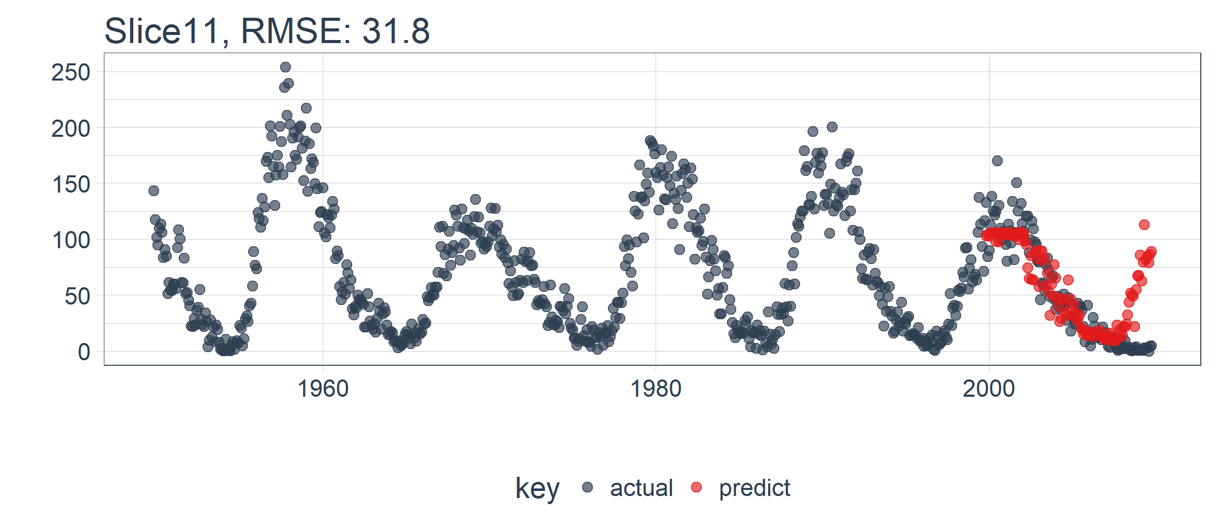
LSTM 模型表现相对较好! 我们选择的设置似乎产生了一个不错的模型,可以捕捉到数据中的趋势。预测在下一个上升趋势前抢跑了,但总体上好过了我的预期。现在,我们需要通过回测来查看随着时间推移的真实表现!
5.2 在 11 个样本上回测 LSTM 模型
一旦我们有了能在一个样本上工作的 LSTM 模型,扩展到全部 11 个样本上就相对简单。我们只需创建一个预测函数,再套用到 rolling_origin_resamples 中抽样计划包含的数据上。
5.2.1 构建一个 LSTM 预测函数
这一步看起来很吓人,但实际上很简单。我们将 5.1 节的代码复制到一个函数中。我们将它作为一个安全函数,对于任何长时间运行的函数来说,这是一个很好的做法,可以防止单个故障停止整个过程。
predict_keras_lstm <- function(split,
                               epochs = 300,
                               ...) {

    lstm_prediction <- function(split,
                                epochs,
                                ...) {

        # 5.1.2 Data Setup
        df_trn <- training(split)
        df_tst <- testing(split)

        df <- bind_rows(
            df_trn %>% add_column(key = "training"),
            df_tst %>% add_column(key = "testing")) %>%
            as_tbl_time(index = index)

        # 5.1.3 Preprocessing
        rec_obj <- recipe(value ~ ., df) %>%
            step_sqrt(value) %>%
            step_center(value) %>%
            step_scale(value) %>%
            prep()

        df_processed_tbl <- bake(rec_obj, df)

        center_history <- rec_obj$steps[[2]]$means["value"]
        scale_history  <- rec_obj$steps[[3]]$sds["value"]

        # 5.1.4 LSTM Plan
        lag_setting  <- 120 # = nrow(df_tst)
        batch_size   <- 40
        train_length <- 440
        tsteps       <- 1
        epochs       <- epochs

        # 5.1.5 Train/Test Setup
        lag_train_tbl <- df_processed_tbl %>%
            mutate(
                value_lag = lag(value, n = lag_setting)) %>%
            filter(!is.na(value_lag)) %>%
            filter(key == "training") %>%
            tail(train_length)

        x_train_vec <- lag_train_tbl$value_lag
        x_train_arr <- array(
            data = x_train_vec, dim = c(length(x_train_vec), 1, 1))

        y_train_vec <- lag_train_tbl$value
        y_train_arr <- array(
            data = y_train_vec, dim = c(length(y_train_vec), 1))

        lag_test_tbl <- df_processed_tbl %>%
            mutate(
                value_lag = lag(value, n = lag_setting)) %>%
            filter(!is.na(value_lag)) %>%
            filter(key == "testing")

        x_test_vec <- lag_test_tbl$value_lag
        x_test_arr <- array(
            data = x_test_vec, dim = c(length(x_test_vec), 1, 1))

        y_test_vec <- lag_test_tbl$value
        y_test_arr <- array(
            data = y_test_vec, dim = c(length(y_test_vec), 1))

        # 5.1.6 LSTM Model
        model <- keras_model_sequential()

        model %>%
            layer_lstm(
                units            = 50,
                input_shape      = c(tsteps, 1),
                batch_size       = batch_size,
                return_sequences = TRUE,
                stateful         = TRUE) %>%
            layer_lstm(
                units            = 50,
                return_sequences = FALSE,
                stateful         = TRUE) %>%
            layer_dense(units = 1)

        model %>%
            compile(loss = 'mae', optimizer = 'adam')

        # 5.1.7 Fitting LSTM
        for (i in 1:epochs) {
            model %>%
                fit(x          = x_train_arr,
                    y          = y_train_arr,
                    batch_size = batch_size,
                    epochs     = 1,
                    verbose    = 1,
                    shuffle    = FALSE)

            model %>% reset_states()
            cat("Epoch: ", i)
        }

        # 5.1.8 Predict and Return Tidy Data
        # Make Predictions
        pred_out <- model %>%
            predict(x_tes