t_arr, batch_size = batch_size) %>%
.[,1]
# Retransform values
pred_tbl <- tibble(
index = lag_test_tbl$index,
value = (pred_out * scale_history + center_history)^2)
# Combine actual data with predictions
tbl_1 <- df_trn %>%
add_column(key = "actual")
tbl_2 <- df_tst %>%
add_column(key = "actual")
tbl_3 <- pred_tbl %>%
add_column(key = "predict")
# Create time_bind_rows() to solve dplyr issue
time_bind_rows <- function(data_1, data_2, index) {
index_expr <- enquo(index)
bind_rows(data_1, data_2) %>%
as_tbl_time(index = !! index_expr)
}
ret <- list(tbl_1, tbl_2, tbl_3) %>%
reduce(time_bind_rows, index = index) %>%
arrange(key, index) %>%
mutate(key = as_factor(key))
return(ret)
}
safe_lstm <- possibly(lstm_prediction, otherwise = NA)
safe_lstm(split, epochs, ...)
}
我们测试下 predict_keras_lstm() 函数,设置 epochs = 10。返回的数据为长格式,在 key 列中标记有 actual 和 predict。
predict_keras_lstm(split, epochs = 10)
## # A time tibble: 840 x 3
## # Index: index
##    index      value key
##    <date>     <dbl> <fct>
##  1 1949-11-01 144.  actual
##  2 1949-12-01 118.  actual
##  3 1950-01-01 102.  actual
##  4 1950-02-01  94.8 actual
##  5 1950-03-01 110.  actual
##  6 1950-04-01 113.  actual
##  7 1950-05-01 106.  actual
##  8 1950-06-01  83.6 actual
##  9 1950-07-01  91.0 actual
## 10 1950-08-01  85.2 actual
## # ... with 830 more rows
5.2.2 将 LSTM 预测函数应用到 11 个样本上
既然 predict_keras_lstm() 函数可以在一个样本上运行,我们现在可以借助使用 mutate() 和 map() 将函数应用到所有样本上。预测将存储在名为 predict 的列中。注意,这可能需要 5-10 分钟左右才能完成。
sample_predictions_lstm_tbl <- rolling_origin_resamples %>%
     mutate(predict = map(splits, predict_keras_lstm, epochs = 300))
现在,我们得到了 11 个样本的预测,数据存储在列 predict 中。
sample_predictions_lstm_tbl
## # Rolling origin forecast resampling
## # A tibble: 11 x 3
##    splits       id      predict
##  * <list>       <chr>   <list>
##  1 <S3: rsplit> Slice01 <tibble [840 x 3]>
##  2 <S3: rsplit> Slice02 <tibble [840 x 3]>
##  3 <S3: rsplit> Slice03 <tibble [840 x 3]>
##  4 <S3: rsplit> Slice04 <tibble [840 x 3]>
##  5 <S3: rsplit> Slice05 <tibble [840 x 3]>
##  6 <S3: rsplit> Slice06 <tibble [840 x 3]>
##  7 <S3: rsplit> Slice07 <tibble [840 x 3]>
##  8 <S3: rsplit> Slice08 <tibble [840 x 3]>
##  9 <S3: rsplit> Slice09 <tibble [840 x 3]>
## 10 <S3: rsplit> Slice10 <tibble [840 x 3]>
## 11 <S3: rsplit> Slice11 <tibble [840 x 3]>
5.2.3 评估回测表现
通过将 calc_rmse() 函数应用到 predict 列上,我们可以得到所有样本的 RMSE。
sample_rmse_tbl <- sample_predictions_lstm_tbl %>%
    mutate(rmse = map_dbl(predict, calc_rmse)) %>%
    select(id, rmse)

sample_rmse_tbl
## # Rolling origin forecast resampling
## # A tibble: 11 x 2
##    id       rmse
##  * <chr>   <dbl>
##  1 Slice01  48.2
##  2 Slice02  17.4
##  3 Slice03  41.0
##  4 Slice04  26.6
##  5 Slice05  22.2
##  6 Slice06  49.0
##  7 Slice07  18.1
##  8 Slice08  54.9
##  9 Slice09  28.0
## 10 Slice10  38.4
## 11 Slice11  34.2
sample_rmse_tbl %>%
    ggplot(aes(rmse)) +
    geom_histogram(
        aes(y = ..density..),
        fill = palette_light()[[1]], bins = 16) +
    geom_density(
        fill = palette_light()[[1]], alpha = 0.5) +
    theme_tq() +
    ggtitle("Histogram of RMSE")
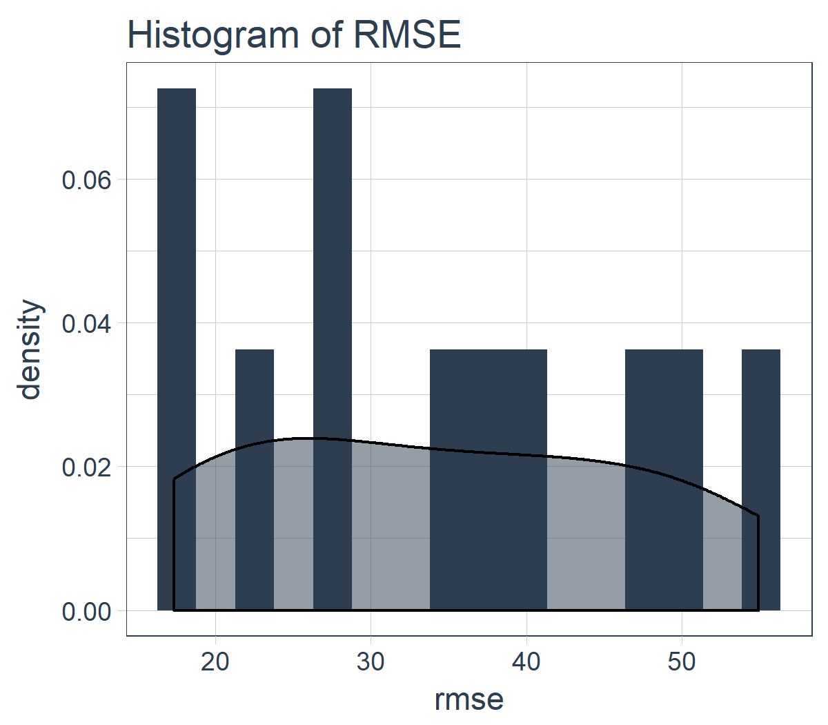
而且,我们可以总结 11 个样本的 RMSE。专业提示:使用 RMSE(或其他类似指标)的平均值和标准差是比较各种模型表现的好方法。
sample_rmse_tbl %>%
    summarize(
        mean_rmse = mean(rmse),
        sd_r