翻译自《Demo Week: Time Series Machine Learning with h2o and timetk》
原文链接:https://www.business-science.io/code-tools/2017/10/28/demo_week_h2o.html
文字和代码略有删改
时间序列分析工具箱―― h2o + timetk
h2o 的用途
h2o 包是 H2O.ai 提供的产品,包含许多先进的机器学习算法,表现指标和辅助函数,使机器学习功能强大而且容易使用。h2o 的主要优点之一是它可以部署在集群上(今天不会讨论),从 R 的角度来看,有四个主要用途:
- 数据操作:拼接、分组、旋转、传输、拆分成训练 / 测试 / 验证集,等等。
- 机器学习算法:包含非常复杂的监督和非监督学习算法。监督学习算法包括深度学习(神经网络)、随机森林、广义线性模型、梯度增强机、朴素贝叶斯分析、模型堆叠集成和 xgboost;无监督算法包括广义低秩模型、k 均值模型和 PCA;还有 Word2vec 用于文本分析。最新的稳定版本还有 AutoML――自动机器学习,我们将在这篇文章中看到这个非常酷的功能!
- 辅助机器学习功能:表现分析和超参数网格搜索。
- 产品、MapReduce 和 云:Java 环境下进行产品化;使用 Hadoop / Spark(Sparkling Water)进行集群部署;在云环境(Azure、AWS、Databricks 等)中部署。
我们将讨论如何将 h2o 用作时间序列机器学习的一种高级算法。我们将在本地使用 h2o,在先前关于 timetk 和 sweep 的教程中使用的数据集(beer_sales_tbl)上开发一个高精度的时间序列模型。这是一个监督学习的回归问题。
加载包
我们需要三个包:
h2o:机器学习算法包tidyquant:用于获取数据和加载tidyverse系列工具timetk:R 中的时间序列工具箱
安装 h2o
推荐在 ubuntu 环境下安装最新稳定版 h2o。
加载包
# Load libraries
library(h2o)        # Awesome ML Library
library(timetk)     # Toolkit for working with time series in R
library(tidyquant)  # Loads tidyverse, financial pkgs, used to get data
数据
我们使用 tidyquant 的函数 tq_get(),获取 FRED 的数据――啤酒、红酒和蒸馏酒销售。
# Beer, Wine, Distilled Alcoholic Beverages, in Millions USD
beer_sales_tbl <- tq_get(
    "S4248SM144NCEN",
    get = "economic.data",
    from = "2010-01-01",
    to = "2017-10-27")

beer_sales_tbl
## # A tibble: 92 x 2
## date price
## <date> <int>
## 1 2010-01-01 6558
## 2 2010-02-01 7481
## 3 2010-03-01 9475
## 4 2010-04-01 9424
## 5 2010-05-01 9351
## 6 2010-06-01 10552
## 7 2010-07-01 9077
## 8 2010-08-01 9273
## 9 2010-09-01 9420
## 10 2010-10-01 9413
## # ... with 82 more rows可视化是一个好主意,我们要知道我们正在使用的是什么数据,这对于时间序列分析和预测尤为重要,并且最好将数据分成训练、测试和验证集。
# Plot Beer Sales with train, validation, and test sets shown
beer_sales_tbl %>%
    ggplot(aes(date, price)) +
    # Train Region
    annotate(
        "text",
        x = ymd("2012-01-01"), y = 7000,
        color = palette_light()[[1]],
        label = "Train Region") +
    # Validation Region
    geom_rect(
        xmin = as.numeric(ymd("2016-01-01")),
        xmax = as.numeric(ymd("2016-12-31")),
        ymin = 0, ymax = Inf, alpha = 0.02,
        fill = palette_light()[[3]]) +
    annotate(
        "text",
        x = ymd("2016-07-01"), y = 7000,
        color = palette_light()[[1]],
        label = "Validation\nRegion") +
    # Test Region
    geom_rect(
        xmin = as.numeric(ymd("2017-01-01")),
        xmax = as.numeric(ymd("2017-08-31")),
        ymin = 0, ymax = Inf, alpha = 0.02,
        fill = palette_light()[[4]]) +
    annotate(
        "text",
        x = ymd("2017-05-01"), y = 7000,
        color = palette_light()[[1]],
        label = "Test\nRegion") +
    # Data
    geom_line(col = palette_light()[1]) +
    geom_point(col = palette_light()[1]) +
    geom_ma(ma_fun = SMA, n = 12, size = 1) +
    # Aesthetics
    theme_tq() +
    scale_x_date(
        date_breaks = "1 year",
        date_labels = "%Y") +
    labs(title = "Beer Sales: 2007 through 2017",
subtitle = "Train, Validation, and Test Sets Shown") 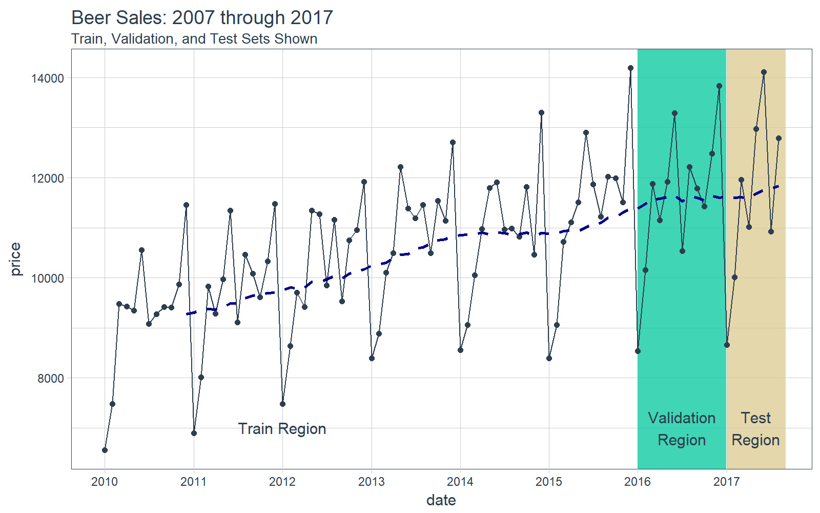
现在我们对数据有了直观的认识,让我们继续吧。
教程:h2o + timetk,时间序列机器学习
我们的时间序列机器学习项目遵循的工作流与之前 timetk + 线性回归文章中的类似。但是,这次我们将用 h2o.autoML() 替换 lm() 函数以获得更高的准确性。
时间序列机器学习
时间序列机器学习是预测时间序列数据的好方法,在开