STEP 2A：ARIMA 模型

我们使用 forecast 包里的 auto.arima() 函数为时间序列建模。

# Model using auto.arima
fit_arima <- auto.arima(beer_sales_ts)

fit_arima

## Series: beer_sales_ts 
## ARIMA(3,0,0)(1,1,0)[12] with drift 
## 
## Coefficients:
##           ar1     ar2     ar3     sar1    drift
##       -0.2498  0.1079  0.6210  -0.2817  32.1157
## s.e.   0.0933  0.0982  0.0925   0.1333   5.8882
## 
## sigma^2 estimated as 175282:  log likelihood=-535.49
## AIC=1082.97   AICc=1084.27   BIC=1096.63

STEP 2B：简化模型

就像 broom 简化 stats 包的使用一样，我么可以使用 sweep 的函数简化 ARIMA 模型。下面介绍三个函数：

• sw_tidy()：用于检索模型参数
• sw_glance()：用于检索模型描述和训练集的精确度度量
• sw_augment()：用于获得模型残差

sw_tidy

sw_tidy() 函数以 tibble 对象的形式返回模型参数。

# sw_tidy - Get model coefficients
sw_tidy(fit_arima)

## # A tibble: 5 x 2
##    term   estimate
##   <chr>      <dbl>
## 1   ar1 -0.2497937
## 2   ar2  0.1079269
## 3   ar3  0.6210345
## 4  sar1 -0.2816877
## 5 drift 32.1157478

sw_glance

sw_glance() 函数以 tibble 对象的形式返回训练集的精确度度量。可以使用 glimpse 函数美化显示结果。

# sw_glance - Get model description and training set accuracy measures
sw_glance(fit_arima) %>%
    glimpse()

## Observations: 1
## Variables: 12
## $ model.desc <chr> "ARIMA(3,0,0)(1,1,0)[12] with drift"
## $ sigma      <dbl> 418.6665
## $ logLik     <dbl> -535.4873
## $ AIC        <dbl> 1082.975
## $ BIC        <dbl> 1096.635
## $ ME         <dbl> 1.189875
## $ RMSE       <dbl> 373.9091
## $ MAE        <dbl> 271.7068
## $ MPE        <dbl> -0.06716239
## $ MAPE       <dbl> 2.526077
## $ MASE       <dbl> 0.4989005
## $ ACF1       <dbl> 0.02215405

sw_augument

sw_augument() 函数返回的 tibble 表中包含 .actual、.fitted 和 .resid 列，有助于在训练集上评估模型表现。注意，设置 timetk_idx = TRUE 返回初始的日期索引。

# sw_augment - get model residuals
sw_augment(fit_arima, timetk_idx = TRUE)

## # A tibble: 84 x 4
##         index .actual   .fitted    .resid
##        <date>   <dbl>     <dbl>     <dbl>
##  1 2010-01-01    6558  6551.474  6.525878
##  2 2010-02-01    7481  7473.583  7.416765
##  3 2010-03-01    9475  9465.621  9.378648
##  4 2010-04-01    9424  9414.704  9.295526
##  5 2010-05-01    9351  9341.810  9.190414
##  6 2010-06-01   10552 10541.641 10.359293
##  7 2010-07-01    9077  9068.148  8.852178
##  8 2010-08-01    9273  9263.984  9.016063
##  9 2010-09-01    9420  9410.869  9.130943
## 10 2010-10-01    9413  9403.908  9.091831
## # ... with 74 more rows

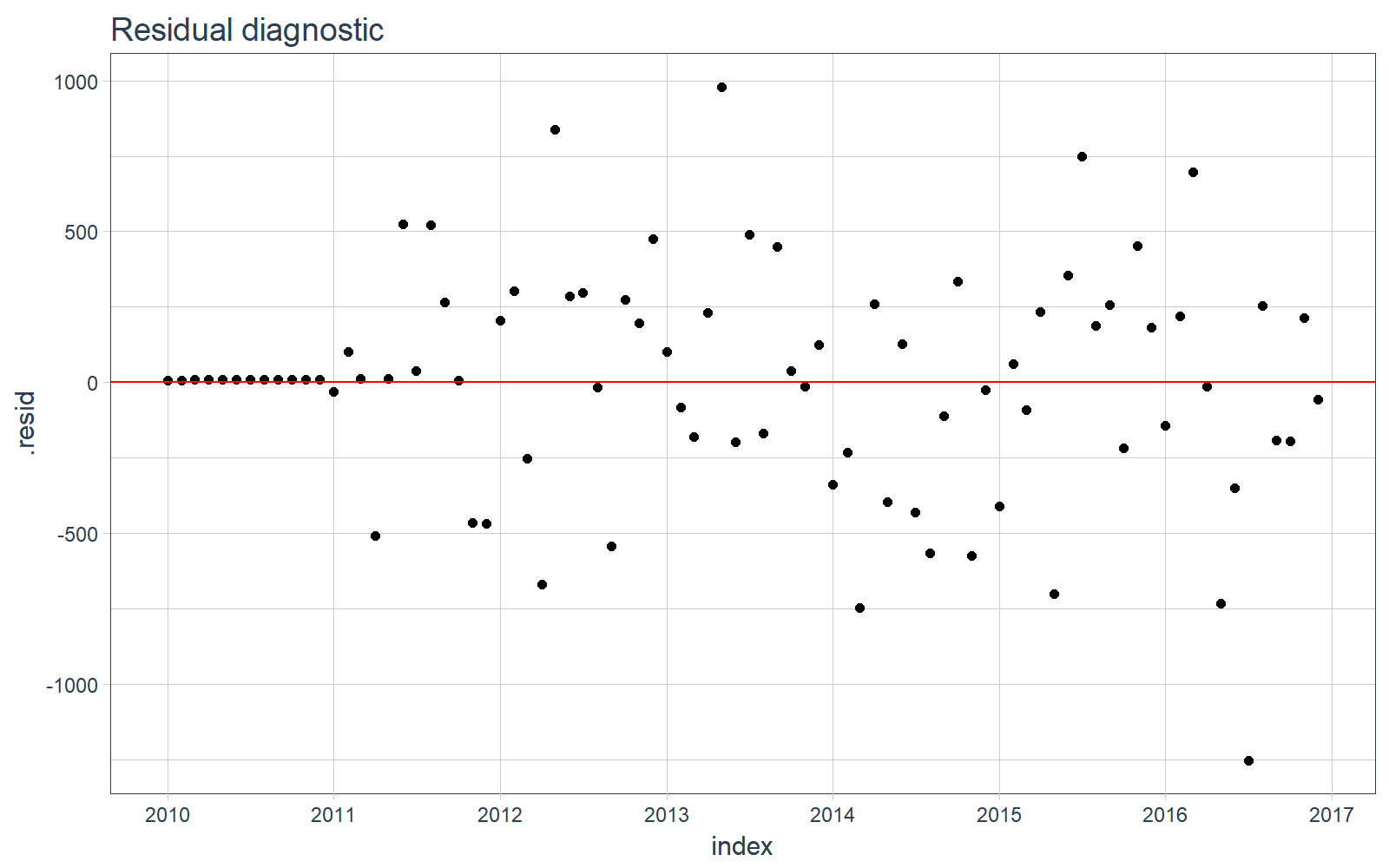
我们可以可视化训练数据上的残差，看一下数据中有没有遗漏的模式没有被发现。

# Plotting residuals
sw_augment(fit_arima, timetk_idx = TRUE) %>%
    ggplot(aes(x = index, y = .resid)) +
    geom_point() + 
    geom_hline(yintercept = 0, color = "red") + 
    labs(title = "Residual diagnostic") +
    scale_x_date(date_breaks = "1 year", date_labels = "%Y") +
    theme_tq()

STEP 3：预测

使用 forecast() 函数做预测。

# Forecast next 12 months
fcast_arima <- forecast(fit_arima, h = 12)

一个问题是，预测结果并不“tidy”。我们需要数据框形式的预测结果，以便应用 tidyverse 的功能，然而预测结果是 forecast 类型的，一种基于 ts 的对象。

class(fcast_arima)

## [1] "forecast"

STEP 4：用 sweep 简化预测

我们使用 sw_sweep() 简化预测结果，一个额外的好处是，如果 forecast 对象有 timetk 索引，我们可以用它返回一个日期时间索引，不同于 ts 对象的规则索引。

首先要确认 forecast 对象有 timetk 索引，这需要在使用 sw_sweep() 时设置 timetk_idx 参数。

# Check if object has timetk index 
has_timetk_idx(fcast_arima)

## [1] TRUE

现在，使用 sw_sweep() 来简化预测结果，它会在内部根据 time_tk 构造一条未来时间序列索引（这一步总是会被执行，因为我们在第 1 步中用 tk_ts() 构造了 ts 对象）注意：这意味着我们最终可以在 forecast 包中使用日期（不同于 ts 对象中的规则索引）！。

# sw_sweep - tidies forecast output
fcast_tbl <- sw_sweep(fcast_arima, timetk_idx = TRUE)

fcast_tbl