mse = sd(rmse))
## # Rolling origin forecast resampling
## # A tibble: 1 x 2
## mean_rmse sd_rmse
## <dbl> <dbl>
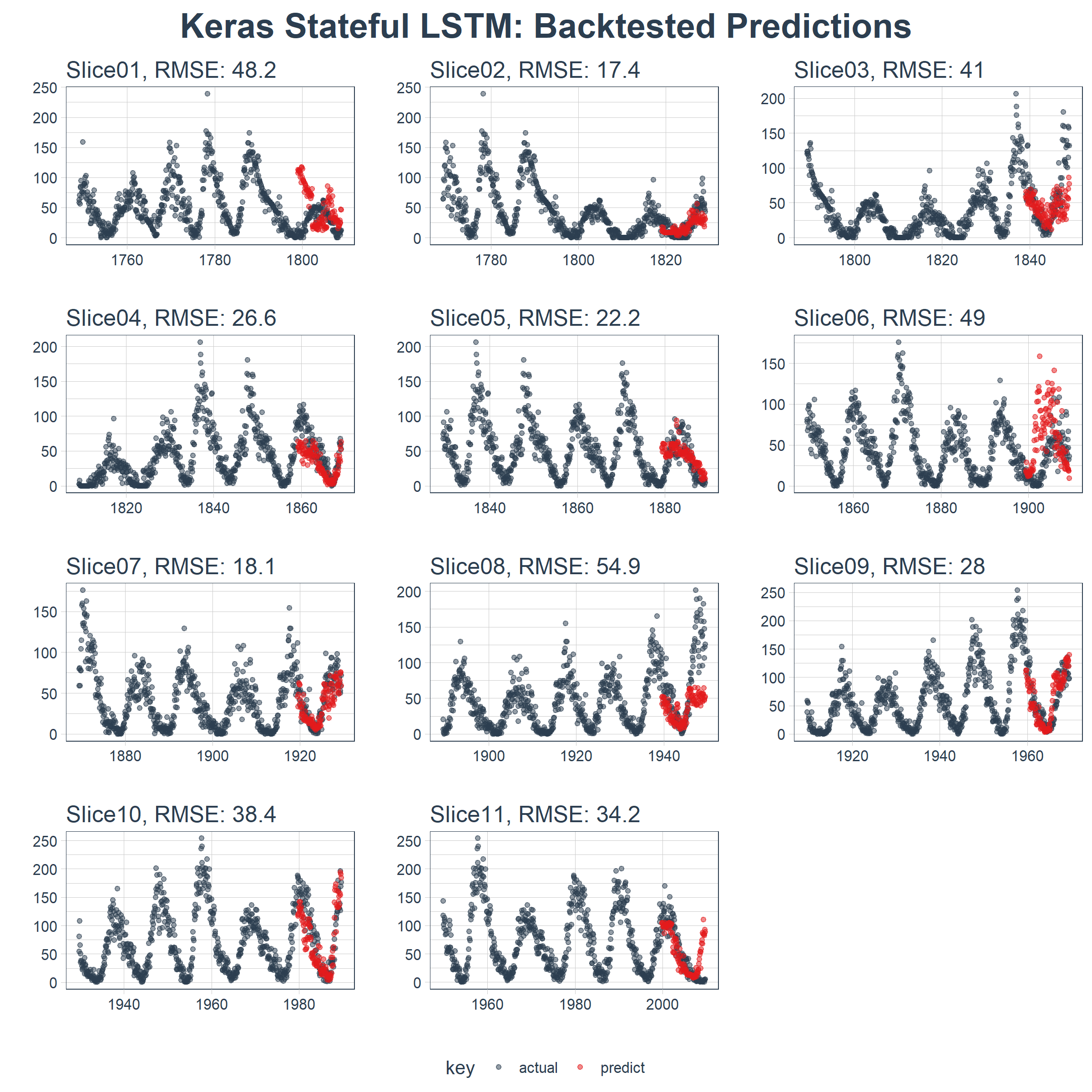
## 1 34.4 13.0
5.2.4 可视化回测的结果
我们可以创建一个 plot_predictions() 函数,把 11 个回测样本的预测结果绘制在一副图上!!!
plot_predictions <- function(sampling_tbl,
                             predictions_col,
                             ncol = 3,
                             alpha = 1,
                             size = 2,
                             base_size = 14,
                             title = "Backtested Predictions") {

    predictions_col_expr <- enquo(predictions_col)

    # Map plot_split() to sampling_tbl
    sampling_tbl_with_plots <- sampling_tbl %>%
        mutate(
            gg_plots = map2(
                !! predictions_col_expr, id,
                .f        = plot_prediction,
                alpha     = alpha,
                size      = size,
                base_size = base_size))

    # Make plots with cowplot
    plot_list <- sampling_tbl_with_plots$gg_plots

    p_temp <- plot_list[[1]] + theme(legend.position = "bottom")
    legend <- get_legend(p_temp)

    p_body  <- plot_grid(plotlist = plot_list, ncol = ncol)


    p_title <- ggdraw() +
        draw_label(
            title,
            size = 18,
            fontface = "bold",
            colour = palette_light()[[1]])

    g <- plot_grid(
        p_title,
        p_body,
        legend,
        ncol = 1,
        rel_heights = c(0.05, 1, 0.05))

    return(g)
}
结果在这里。在一个不容易预测的数据集上,这是相当令人印象深刻的!
sample_predictions_lstm_tbl %>%
    plot_predictions(
        predictions_col = predict,
        alpha = 0.5,
        size = 1,
        base_size = 10,
        title = "Keras Stateful LSTM: Backtested Predictions")
5.3 预测未来 10 年的数据
我们可以通过调整预测函数来使用完整的数据集预测未来 10 年的数据。新函数 predict_keras_lstm_future() 用来预测未来 120 步(或 10 年)的数据。
predict_keras_lstm_future <- function(data,
                                      epochs = 300,
                                      ...) {

    lstm_prediction <- function(data,
                                epochs,
                                ...) {

        # 5.1.2 Data Setup (MODIFIED)
        df <- data

        # 5.1.3 Preprocessing
        rec_obj <- recipe(value ~ ., df) %>%
            step_sqrt(value) %>%
            step_center(value) %>%
            step_scale(value) %>%
            prep()

        df_processed_tbl <- bake(rec_obj, df)

        center_history <- rec_obj$steps[[2]]$means["value"]
        scale_history  <- rec_obj$steps[[3]]$sds["value"]

        # 5.1.4 LSTM Plan
        lag_setting  <- 120 # = nrow(df_tst)
        batch_size   <- 40
        train_length <- 440
        tsteps       <- 1
        epochs       <- epochs

        # 5.1.5 Train Setup (MODIFIED)
        lag_train_tbl <- df_processed_tbl %>%
            mutate(
                value_lag = lag(value, n = lag_setting)) %>%
            filter(!is.na(value_lag)) %>%
            tail(train_length)

        x_train_vec <- lag_train_tbl$value_lag
        x_train_arr <- array(
            data = x_train_vec, dim = c(length(x_train_vec), 1, 1))

        y_train_vec <- lag_train_tbl$value
        y_train_arr <- array(
            data = y_train_vec, dim = c(length(y_train_vec), 1))

        x_test_vec <- y_train_vec %>% tail(lag_setting)
        x_test_arr <- array(
            data = x_test_vec, dim = c(length(x_test_vec), 1, 1))

        # 5.1.6 LSTM Model
        model <- keras_model_sequential()

        model %>%
            layer_lstm(
                units            = 50,
                input_shape      = c(tsteps, 1),
                batch_size       = batch_size,
                return_sequences = TRUE,
                stateful         = TRUE) %>%
            layer_lstm(
                units            = 50,
                return_sequences = FALSE,
                stateful         = TRUE) %>%
            layer_dense(units = 1)

        model %>%
            compile(loss = 'mae', optimizer = 'adam')

        # 5.1.7 Fitting LSTM
        for (i in 1:epochs) {
            model %>%
                fit(x          = x_train_arr,
                    y          = y_train_arr,
                    batch_size = batch_size,
                    epochs     = 1,
                    verbose    = 1,
                    shuffle    = FALSE)

            model %>% reset_states()
            cat("Epoch: ", i)
        }

        # 5.1.8 Predict and Return Tidy Data (MODIFIED)
        # Make Predictions
        pred_out <- model %>%
            predict(x_test_arr, batch_